
ADS-B data#
Can standard geospatial tools be used with transmissions from Automatic Dependent Surveillance-Broadcast (ADS-B) equipment aboard aircraft? I wanted to find out because unlike most geospatial data, ADS-B has a third dimension and a fourth dimension.
My geospatial analysis tool of choice is PostGIS, which has multidimensional geometry types and functions, but I had never really had cause to use them despite having coded support for additional dimensions when I developed plpygis.
This article describes the process of getting free ADS-B data, loading it into PostgreSQL and then manipulating it with PostGIS and Python. Much (but not all!) of this was part of my FOSS4G 2023 talk “Aircraft trajectory analysis using PostGIS”, which was recorded and made available by the organizers.
Tools#
In addition to PostgreSQL and PostGIS, I used two Python modules: requests and plpygis. These must be installed in a location from which PostgreSQL’s PL/Python can import them. I also used QGIS for visualization.
Aircraft identities#
Step one was learning about ICAO 24 addresses, unique aircraft identifiers which are included in every ADS-B transmission.1 These are 24-bit values represented by a six-digit hexadecimal number, such as A4DA1. These codes are distinct from the registration numbers that are visible on an aircraft’s body or tail.

A single physical aircraft may have multiple ICAO 24 addresses over its lifetime but these change much less frequently than registration numbers.
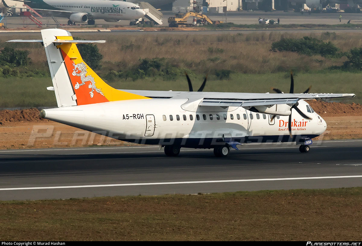
The ATR-42 in the image above has moved between three airlines and therefore been registered under three different numbers … but also with two different ICAO 24 codes, 3a2270 and 39ad00. The history of these alterations can be found in some databases, such as the one maintained by Planespotters.net.
The OpenSky Network#
The The OpenSky Network provides free access to ADB-S data via a RESTful API. There is a Python client, but I did not use it since it doesn’t implement everything that is available directly through the API.2
Anyone may create an OpenSky account as long as they follow the site’s terms of use.
State vectors#
Equipped with an ICAO 24 number, I retrieved some actual flight data provided by OpenSky.3 A basic query also requires a specific time, with that time being represented as the number of seconds elapsed since the 1st of January 1970 (otherwise known as UNIX time). For example, the position of the ATR-42 above at 16:01:23 on the 11th of April, 2022 is requested by https://opensky-network.org/api/states/all?icao24=39ad00&time=1649692883.
The JSON-encoded response looks like the following:
{
  "time": 1649692883,
  "states": [
    [
      "39ad00",
      "AFR57AG ",
      "France",
      1649692879,
      1649692882,
      2.5172,
      44.9426,
      2263.14,
      false,
      100.86,
      24.08,
      10.08,
      null,
      2316.48,
      null,
      false,
      0
    ]
  ]
}
The data transmitted by the aircraft is stored in the list of states and can be decoded through the OpenSky documentation. From this you know that the aircraft was operating as Air France 57AG, that it recorded a barometric altitude of 2263.14 meters, that it had a ground speed of 100.86 meters/second and so on.
Tracks#
OpenSky simplifies getting a series of state vectors by providing a tracks API endpoint, and although the documentation states that this endpoint is experimental, I’ve had success in using it: https://opensky-network.org/api/tracks/?icao24=39ad00&time=1649692883.
The response to the request above will contain some basic facts about the flight, including the first and last times at which it was observed:
{
  "icao24": "39ad00",
  "callsign": "AFR57AG ",
  "startTime": 1649692883,
  "endTime": 1649696435,
  "path": [...]
}
The path element is a list of abbreviated state vectors showing the route the aircraft took on this flight. One of these vectors might look like the following:
[
  1649693075,
  45.129,
  2.631,
  3352,
  23,
  false
]
These values are the time, latitude, longitude, barometric altitude, heading and whether the aircraft is on the ground respectively. Note that the latitude/longitude ordering switches between the /states and /tracks endpoints! One other thing to be aware of is that tracks in OpenSky are reported in 1000 foot steps, so aircraft will appear to take off from an altitude of 0m and proceed to an elevation of 304m, then 609m and so on.4 See the Appendix for a function to do this.
The one significant limitation with OpenSky is that these flight tracks are only available for flights from the last 30 days.
Flights#
The next endpoint that we’ll be using is /flights/aircraft, which lists all the flights taken by an aircraft: https://opensky-network.org/api/flights/aircraft/?icao24=39ad00&begin=1609455600&end=1609714800.
One flight in the list looks like the following:
{
  "icao24": "39ad00",
  "firstSeen": 1649692883,
  "estDepartureAirport": "LFLW",
  "lastSeen": 1649696438,
  "estArrivalAirport": "LFPO",
  "callsign": "AFR57AG ",
  "estDepartureAirportHorizDistance": 9750,
  "estDepartureAirportVertDistance": 1654,
  "estArrivalAirportHorizDistance": 3750,
  "estArrivalAirportVertDistance": 33,
  "departureAirportCandidatesCount": 0,
  "arrivalAirportCandidatesCount": 9
}
The departure and arrival airports are estimates since these are not explicitly reported by the ADB-S data, so OpenSky infers them from what it observes; on occasion you will see an airport listed as null when there wasn’t enough data to establish what the plane’s origin or destination were.
Any time between firstSeen and lastSeen can be used with the /tracks endpoint above to get the entire path that the plane took on this flight.
Airport activity#
Two final endpoints that are interesting are /flights/arrival and /flights/departure, which will list all the flights that terminate or originate at a particular airport between two points in time.
ADS-B data in PostGIS#
Database creation#
Once PostgreSQL and PostGIS are installed and your user has the right privileges, you can run the following on the command line:
createdb opensky
Then open the database to interact with it:
pgsql opensky
You first need to enable PostGIS:
CREATE EXTENSION postgis;
Create the table to store the flight data:
CREATE TABLE flight (
  icao24   TEXT,
  callsign TEXT,
  airport_depart TEXT,
  airport_arrive TEXT,
  time_depart TIMESTAMP,
  time_arrive TIMESTAMP,
  geom GEOMETRY(LINESTRINGZM, 4326)
);
The geometry type LINESTRINGZM means that each vertex in the path will have four dimensions: x and y (longitude and latitude), z (altitude) and m (the “measure” value, which will be used for time).
Finally, add an index but make it n-dimensional, which optimizes queries across all four dimensions.
CREATE INDEX ON
  flight
USING
  gist (geom gist_geometry_ops_nd);
PL/Python#
There are a few ways to bring the data from the OpenSky API into the database, but I used PL/Python, which means we’ll write a function in Python that will be run from inside the database. To make it easier to work with PostGIS, I also used plpygis, a small Python module that I created to help write PL/Python functions for geospatial data.
Start by enabling PL/Python:
CREATE LANGUAGE plpython3u;
Let’s start with a simple function that gets a list of flights an aircraft took between two dates. I provided my OpenSky credentials in the environment variables OPENSKY_USER and OPENSKY_PASS, but they could also be set directly in the script.5
CREATE OR REPLACE FUNCTION
    opensky_get_aircraft_flights(icao24 TEXT, in_datebegin DATE, in_dateend DATE)
RETURNS
    TABLE (LIKE flight)
AS $$
    import os
    OSUSER = os.getenv("OPENSKY_USER")
    OSPASS = os.getenv("OPENSKY_PASS")
    OSURL = "https://opensky-network.org/api"

    from datetime import datetime
    from dateutil import parser
    from requests import Session
    from requests.auth import HTTPBasicAuth

    db = parser.parse(in_datebegin)
    de = parser.parse(in_dateend).replace(hour=23, minute=59)
    db = int(db.timestamp())
    de = int(de.timestamp())

    opensky = Session()
    opensky.auth = HTTPBasicAuth(OSUSER, OSPASS)

    res = opensky.get(
              OSURL + "/flights/aircraft/",
              params={"icao24" : icao24,
                      "begin" : db,
                      "end" : de})

    if res.status_code == 200 and res.text:
        plpy.info(res.request.url)
        flights = [(icao24,
                    f["callsign"].strip() if f["callsign"] else "",
                    f["estDepartureAirport"],
                    f["estArrivalAirport"],
                    datetime.fromtimestamp(f["firstSeen"]),
                    datetime.fromtimestamp(f["lastSeen"]),
                    None)
                   for f in res.json()]
        return flights
    else:
        plpy.info(res.request.url, res.status_code, res.text)
        return []

$$ LANGUAGE plpython3u;
The function definition opensky_get_aircraft_flights takes three arguments, the ICAO 24 code discussed above plus a start and an end date. Returning TABLE (LIKE flight) is a rather useful way that PostgreSQL lets you force the output of a function to match exactly the definition of a table.6
The function makes a call to the OpenSky API to get all the flights for the aircraft between the two dates, and returns the results. It does not fill in the track for each flight, but we can write another function to do that:
CREATE OR REPLACE FUNCTION
    opensky_get_track(icao24 TEXT, in_date TIMESTAMP WITH TIME ZONE)
RETURNS
    GEOMETRY(LINESTRINGZM, 4326)
AS $$
    import os
    OSUSER = os.getenv("OPENSKY_USER")
    OSPASS = os.getenv("OPENSKY_PASS")
    OSURL = "https://opensky-network.org/api"

    from datetime import datetime
    from dateutil import parser
    from requests import Session
    from requests.auth import HTTPBasicAuth
    from plpygis import LineString

    dt = parser.parse(in_date)
    dt = int(dt.timestamp())

    opensky = Session()
    opensky.auth = HTTPBasicAuth(OSUSER, OSPASS)

    res = opensky.get(
                OSURL + "/tracks/",
                params={"icao24" : icao24.lower(),
                        "time" : dt})
    if res.status_code == 200 and res.text:
        plpy.info(res.request.url)
        fl = res.json()
        return LineString(
                    [[v[2], v[1], v[3], v[0]]
                    for v in fl["path"]])
    else:
        plpy.info(res.request.url, res.status_code, res.text)
        return None
$$ LANGUAGE plpython3u;
Now you can use SQL on the results of this function as if it were a normal database table. For example if you want to know all the unique flight numbers flown by 39ad00 in the first week of May, you can query the OpenSky API like this:
SELECT
  DISTINCT callsign
FROM
  opensky_get_aircraft_flights('c05f01', '2022-05-01', '2022-05-07');
 callsign
----------
 JZA653
 JZA652
 JZA270
 JZA283
 JZA651
 JZA161
 JZA399
 JZA300
 JZA157
 JZA460
 JZA801
 JZA349
 JZA279
 JZA322
 JZA658
 JZA164
 JZA282
 JZA153
 JZA156
 JZA295
 JZA147
 JZA400
 JZA810
 JZA800
 JZA654
 JZA803
 JZA160
 JZA459
One issue that you will observe doing the above is that you are pulling data from the API with every query. It will be much better to have a local copy of the data to work with:
INSERT INTO
  flight
SELECT
  *
FROM
  opensky_get_aircraft_flights('c05f01', '2022-05-01', '2022-05-07');
Now the same queries can be run locally from our flight table:
SELECT DISTINCT
  callsign
FROM
  flight;
And how do we add the tracks?
UPDATE
  flight
SET
  geom = opensky_get_track(icao24, time_depart)
WHERE
  date(time_depart) = '2022-05-01';
Remove the WHERE clause and you’ll add tracks to all the flights in your table (which could take a very long time depending on what you have put in there). To add geometries to all the flights without them, you can change the where clause to WHERE geom IS NULL.
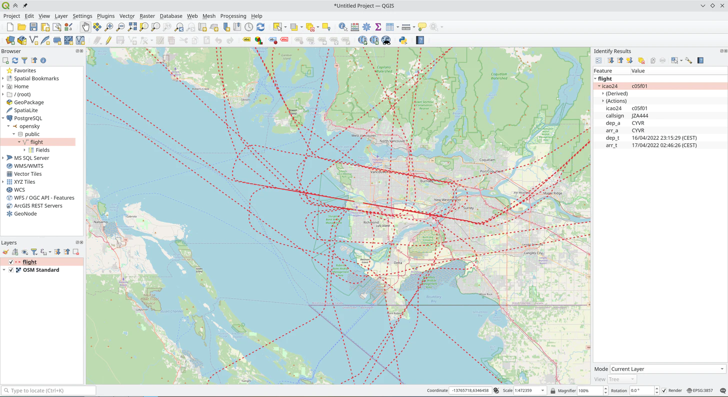
And, of course, you can hook the table up to QGIS to see those flight paths.
Geospatial queries#
With the data in PostGIS, let’s do some analysis.
Let’s start easy and say that you want to know how many kilometers 39ad00 flew on the 1st of May:
SELECT
  count(*) AS flights,
  SUM(ST_Length(geom::geography)) / 1000 AS distance
FROM
  flight
WHERE
  date(time_depart) = '2022-05-01';
 flights |     distance
---------+-------------------
       5 | 1499.689291267288
A little more advanced is seeing how often 39ad00 flew between two Canadian airports but travelled over the landmass of the United States to get there. To do this, I downloaded the administrative boundaries data set from NaturalEarth and after unzipping it, I loaded it into the opensky database:
shp2pgsql -s 4326 -g geom ne_10m_admin_0_countries.shp country | psql opensky
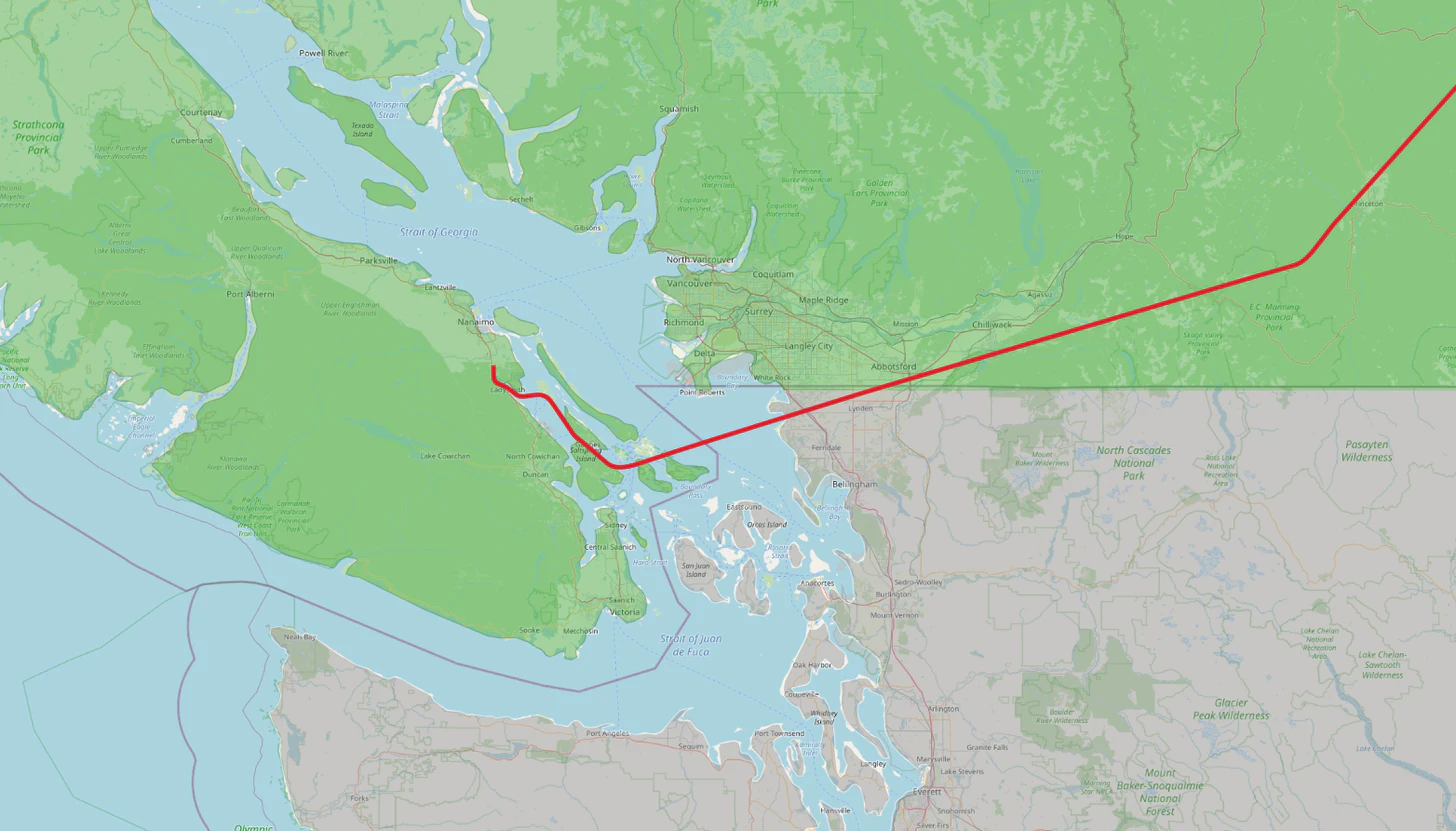
And the I ran the following query to find instances when the start and end of a flight were in Canada but at some point the flight path intersected with US territory:
SELECT
  f.callsign, f.time_depart, f.airport_depart, f.airport_arrive
FROM
  flight AS f, country AS usa, country AS canada
WHERE
  usa.name = 'United States of America' AND
  canada.name = 'Canada' AND
  ST_Intersects(canada.geom, ST_StartPoint(f.geom)) AND
  ST_Intersects(canada.geom, ST_EndPoint(f.geom)) AND
  ST_Intersects(usa.geom, f.geom);
 callsign |      time_depart    | airport_depart | airport_arrive
----------+---------------------+----------------+----------
 JZA474   | 2022-05-13 01:10:16 | CYCD           | CYYC
Showing that particular flight in QGIS, we can see how it did, in fact, pass over the United States during its flight.
Going multidimensional#
Crossed Paths#
With some data in our flight table, we can do multidimensional analysis using three dimensions as described in the PostGIS documentation.
Let’s start by seeing if any of the flights had an exact intersections of their flight paths.
SELECT
  a.callsign, a.time_depart,
  b.callsign, b.time_depart,
  ST_AsText(ST_Intersection(a.geom, b.geom))
FROM
  flight AS a, flight AS b
WHERE
  a.time_depart > b.dep_time AND
  ST_Intersects(ST_Force3D(a.geom), ST_Force3D(b.geom));
Note that we are forcing the geometries to be three-dimensional and not four-dimensional. A two-dimentional intersection would ignore altitude completely, while a four-dimensional intersection would be asking for two planes that crossed paths at the exact same point at the exact same time, otherwise known as a mid-air collision.
Among the results is something like this, where we can see the exact three-dimensional point at which the paths of Jazz Air flights 168 and 150 intersected one another.
JZA168 | 2022-06-07 04:49:17 | JZA150 | 2022-06-06 18:15:24 | POINT Z (-123.28160909937012 48.72753520085094 609)
The intersection point is expressed in three-dimensional WKT, POINT Z (-123.28160909937012 48.72753520085094 609), where the 609 indicates that the planes were at an altitude of 609 metres or about 2000 feet, a reasonable altitude for planes on approach to an airport.
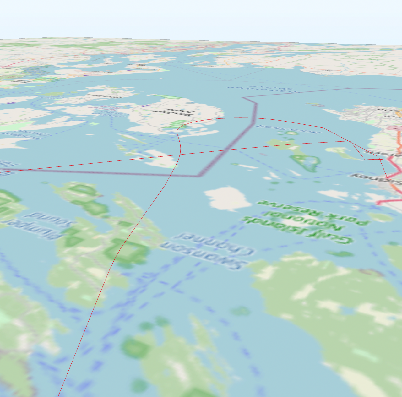
Click here to see the 3d model above (vertical scale has been exaggerated).
Four dimensions#
Closest points of approach#
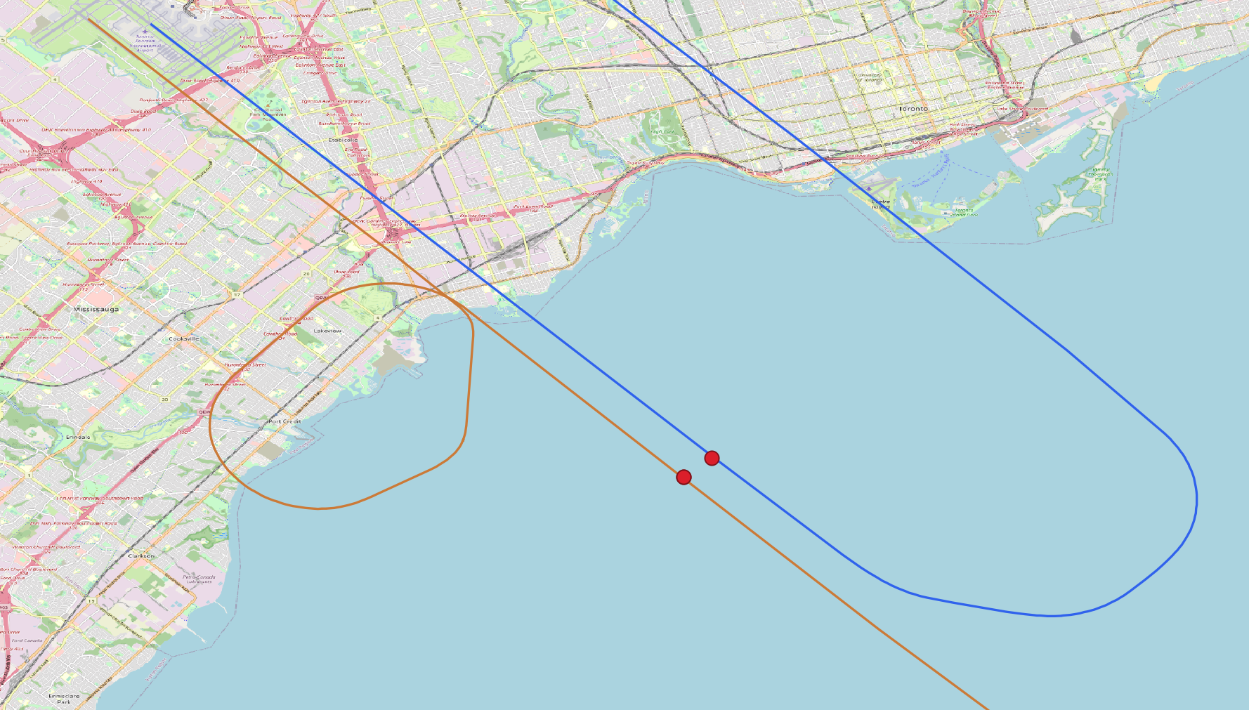
A four-dimensional intersection is a mid-air collision, and Canada’s Civil Aviation Daily Occurrence Reporting System has a queryable database of “occurrences” on the Transport Canada website. By filtering on the string “TCAS”7, I found the following incident:
UPDATE: TSB Report #A22O0076: C-FAXD, a Boeing 737 MAX 8 aircraft operated by Sunwing Airlines Inc, was conducting flight SWG443 from Punta Cana International Airport (PUJ/MDPC), Dominican Republic, to Toronto Pearson International Airport (CYYZ), ON. While on final approach into CYYZ for Runway 33L, the flight crew received a Traffic Alert and Collision Avoidance System (TCAS) resolution advisory (RA) with C-GJVT, an Airbus 320-200 aircraft operated by Air Canada conducting flight ACA264 from Winnipeg/James Armstrong Richardson International Airport (CYWG), MB, to CYYZ, which was on final approach for Runway 33R. SWG443 followed the TCAS RA and aborted the approach to the left. Both aircraft came to a minimum lateral separation of 0.6 Nautical Miles and a minimum vertical separation of 500 feet. SWG443 was at an altitude of 3500 feet and ACA264 at 3000 feet, abeam to each other, on approach for Runways 33L and 33R. SWG443 and ACA264 landed without further incident.
I wanted to see if I could replicate this narrative in ADS-B data. The first problem is that all the data in the flight table comes from the same airplane, so I added a new function that ingests all the tracks arriving or departing from a specific airport.
CREATE OR REPLACE FUNCTION
    opensky_get_airport_flights(airport TEXT, in_datebegin DATE, in_dateend DATE)
RETURNS
    TABLE (LIKE flight)
AS $$
    import os
    OSUSER = os.getenv("OPENSKY_USER")
    OSPASS = os.getenv("OPENSKY_PASS")
    OSURL = "https://opensky-network.org/api"

    from datetime import datetime
    from dateutil import parser
    from requests import Session
    from requests.auth import HTTPBasicAuth

    db = parser.parse(in_datebegin)
    de = parser.parse(in_dateend).replace(hour=23, minute=59)
    db = int(db.timestamp())
    de = int(de.timestamp())

    opensky = Session()
    opensky.auth = HTTPBasicAuth(OSUSER, OSPASS)

    for endpoint in ["arrival", "departure"]:
      res = opensky.get(
                OSURL + "/flights/{}/".format(endpoint),
                params={"airport" : airport,
                        "begin" : db,
                        "end" : de})

      if res.status_code == 200 and res.text:
          plpy.info(res.request.url)
          for f in res.json():
            if not f["firstSeen"] or not f["lastSeen"]:
              continue
            yield (f["icao24"],
                   f["callsign"].strip() if f["callsign"] else "",
                   f["estDepartureAirport"],
                   f["estArrivalAirport"],
                   datetime.fromtimestamp(f["firstSeen"]),
                   datetime.fromtimestamp(f["lastSeen"]),
                   None)
      else:
          plpy.info(res.request.url, res.status_code, res.text)

$$ LANGUAGE plpython3u;
I populated it with the flights to and from CYYZ on the date of the incident.
CREATE TABLE tcas (LIKE flight);
INSERT INTO tcas
SELECT
  *
FROM
  opensky_get_airport_flights('CYYZ', '2022-06-18', '2022-06-18');
I could have ingested all the tracks for every row in the table, but since I already knew the affected flights, I just focused on those.
UPDATE
  tcas
SET
  geom = opensky_get_track(icao24, time_depart)
WHERE
  callsign IN ('ACA264', 'SWG443');
After adding the tracks, the PostGIS function ST_ClosestPointOfApproach can tell us where along the timelines of two flights are they at their closest proximity. We will, however, want to have the geometry reprojected into a spatial reference system that makes distance calculations using metres - not latitude and longitude - since that is what the altitude is measured in. Since the data set is clustered around Toronto, EPSG:7991 is a good choice.
ST_ClosestPointOfApproach finds the measure value at which two tracks are closest to one another. ST_DistanceCPAprovides the actual three-dimensional distance between the two tracks at this closest point of approach.
WITH flights AS (
  SELECT
    a.callsign AS fa,
    b.callsign AS fb,
    ST_Transform(a.geom, 7991) AS ga,
    ST_Transform(b.geom, 7991) AS gb
  FROM
    tcas AS a, tcas AS b
  WHERE
    a.callsign = 'ACA264' AND
    b.callsign = 'SWG443'
), cpa AS (
  SELECT
    fa, fb, ga, gb,
    ST_ClosestPointOfApproach(ga, gb) AS m
  FROM
    flights
), points AS (
  SELECT
    fa,
    fb,
    ST_Force3DZ(ST_GeometryN(ST_LocateAlong(ga, m), 1)) AS pa,
    ST_Force3DZ(ST_GeometryN(ST_LocateAlong(gb, m), 1)) AS pb,
    ST_DistanceCPA(ga, gb) AS distance,
    m
  FROM
    cpa
)
SELECT
  to_timestamp(m) AT TIME ZONE 'UTC' AS time,
  round(distance) AS separation,
  round(ST_Distance(ST_Force2D(pa), ST_Force2D(pb))) AS lateral_separation,
  round(abs(ST_Z(pa) - ST_Z(pb))) AS vertical_separation,
  fa AS a,
  fb AS b,
  ST_AsText(ST_Transform(pa, 4326), 3) AS a_position,
  ST_AsText(ST_Transform(pb, 4326), 3) AS b_position
FROM
  points;
According to Transport Canada, the lateral separation at 22:39 UTC should be 0.6 nautical miles, which is is 1111 metres, and the vertical separation should be approximately 500 feet. The ADS-B data doesn’t exactly replicate those findings but it’s not hugely far off.
        time         | separation | lateral_separation | vertical_separation |   a    |   b    |            a_position            |          b_position
---------------------+------------+--------------------+---------------------+--------+--------+----------------------------------+------------------------------
 2022-06-18 22:38:07 |       1119 |               1075 |                 310 | ACA264 | SWG443 | POINT Z (-79.448 43.542 604.234) | POINT Z (-79.457 43.536 914)
The altitude of the two flights does not match the altitudes stated by Transport Canada; however, the altitude measurement in the tracks is the elevation above ground, so adding ~170m to account for the airport’s elevation does bring us into that range.
Searching for near misses#
Lastly, I wanted to see if there were any “close calls” like the one above that were not reported in the Transport Canada database.
Let’s load the in-bound and out-bound flights at Victoria International Airport (YYJ) on a single day:
INSERT INTO flight
SELECT
  *
FROM
  opensky_get_airport_flights('CYYJ', '2022-06-15', '2022-06-15');
From this we will see for all flights that have any temporal overlap, there is a single time at which the two flights were closest to one another.
SELECT
  to_timestamp(ST_ClosestPointOfApproach(ST_Transform(a.geom, 3005), ST_Transform(b.geom, 3005))) AS time,
  a.callsign AS flight_a,
  b.callsign AS flight_b
FROM
  flight as a, flight as b
WHERE
  a.time_depart > b.dep_time AND
  ST_ClosestPointOfApproach(a.geom, b.geom) IS NOT NULL;
An abbreviated output would look like the following:
             time              | flight_a | flight_b
-------------------------------+----------+----------
 2022-06-15 16:50:34.289124+02 | WSW209   | ROU1901
 2022-06-15 16:13:25+02        | WSW209   | MAL8072
 2022-06-15 16:13:25+02        | WSW209   | WJA209
 2022-06-15 23:20:26+02        | ASP654   | WJA196
 2022-06-15 23:16:29.999995+02 | ASP654   | FLE515
 2022-06-15 23:01:11+02        | ASP654   | CGFHA
 2022-06-15 23:11:15+02        | ASP654   | CL604KGN
 2022-06-15 23:01:03+02        | ASP654   | CGBMO
 2022-06-15 23:11:15+02        | ASP654   | ROU1902
 2022-06-15 23:01:03+02        | ASP654   | CGBMO
Let’s say we want to find instances where two aircraft were within 1000 metres of one another:
WITH flights AS (
  SELECT
    a.callsign AS fa,
    b.callsign AS fb,
    ST_Transform(a.geom, 3005) AS ga,
    ST_Transform(b.geom, 3005) AS gb
  FROM
    flight AS a, flight AS b
  WHERE
    a.time_depart > b.dep_time
), cpa AS (
  SELECT
    fa, fb, ga, gb,
    ST_DistanceCPA(ga,gb) AS sd,
    ST_ClosestPointOfApproach(ga, gb) AS m
  FROM
    flights
  WHERE
    ST_ClosestPointOfApproach(ga, gb) IS NOT NULL
)
SELECT
  m AS unix_time,
  round(sd) AS separation,
  fa AS flight_a,
  fb AS flight_b
FROM
  cpa
WHERE
  sd <= 1000;
This gives us the following output, including one remarkable outlier where two planes were within just 31 metres of one another (at least as reported by the ADS-B data)!
     unix_time      | separation | flight_a | flight_b
--------------------+------------+----------+----------
         1655318221 |        782 | N90422   | N50KA
 1655317602.2365394 |         31 | CGGGO    | WEN3354
  1655246393.916999 |        984 | CGVEA    | CFSUV
 1655253184.6499498 |        996 | CGLDP    | JZA161
A separation of 31 metres is so small that it’s worth double checking the data to see what those two aircraft were doing at exactly 1655317602.2365394.
SELECT ST_AsText(geom)
FROM (
  SELECT (ST_DumpPoints(flight.geom)).*
  FROM flight WHERE callsign = 'CGGGO') AS g;
From the points in flight CGGGO, we see that there were ADS-B state vectors recorded two minutes before and 13 seconds after 1655317602, but no state vector exactly at 1655317602.
  path |                            st_astext
------+-----------------------------------------------------------------
 {1}  | POINT ZM (1218224.1390170476 455564.6965150813 0 1655317419)
 {2}  | POINT ZM (1218370.96000034 455381.88762515073 0 1655317425)
 {3}  | POINT ZM (1218440.9541452834 455284.7816067032 0 1655317428)
 {4}  | POINT ZM (1218456.977321602 455252.1045787118 0 1655317429)
 {5}  | POINT ZM (1218559.022961798 455089.6465681435 0 1655317434)
 {6}  | POINT ZM (1218582.8252591728 455046.18074272043 0 1655317436)
 {7}  | POINT ZM (1218614.8748292197 454980.82785217743 0 1655317437)
 {8}  | POINT ZM (1218623.5907024834 454947.84267283714 0 1655317438)
 {9}  | POINT ZM (1218624.5285217932 454925.6466826303 0 1655317439)
 {10} | POINT ZM (1218634.1823688783 454870.46557313844 0 1655317440)
 {11} | POINT ZM (1218635.5891432345 454837.17162861006 0 1655317441)
 {12} | POINT ZM (1218636.5269924412 454814.975674214 0 1655317442)
 {13} | POINT ZM (1218632.4999741595 454736.98104434885 0 1655317444)
 {14} | POINT ZM (1218627.066055597 454692.2803657774 0 1655317445)
 {15} | POINT ZM (1218598.019306817 454513.16918261163 0 1655317450)
 {16} | POINT ZM (1218524.7346475082 453820.77799814986 0 1655317466)
 {17} | POINT ZM (1218516.20432238 453675.88890926924 0 1655317469)
 {18} | POINT ZM (1218497.63525764 453074.757360585 304 1655317482)
 {19} | POINT ZM (1218212.1383303064 445414.31268528895 609 1655317615)
 {20} | POINT ZM (1218196.3919528325 445091.2794655764 609 1655317620)
 {21} | POINT ZM (1218224.3295626454 442858.135926426 914 1655317663)
 {22} | POINT ZM (1218221.4493862633 441879.82805676176 914 1655317684)
 ...
What PostGIS is doing is interpolating the coordinates when the exact measure value does not exist in the data set:
WITH point AS (
  SELECT
    callsign,
    ST_GeometryN(ST_LocateAlong(ST_Transform(a.geom, 3005), 1655317602.2365394), 1) AS pa
  FROM
    flight AS a
  WHERE
    a.callsign in ('CGGGO', 'WEN3354')
)
SELECT
  callsign,
  ST_AsText(ST_Force3DZ(pa), 0) AS position
FROM
  point;
Compare the results with the table above and you’ll see how the values fit between the two highlighted lines.
 callsign |           position
----------+------------------------------
 CGGGO    | POINT Z (1218240 446149 580)
 WEN3354  | POINT Z (1218249 446149 609)
Apply a little Pythagorean theorem and the distance was, in fact, 31 metres. Well … sort of. Because of gaps in the ADS-B data, all PostGIS can do is estimate where the planes actually were. But if those estimates were correct, then the rest of the math does, in fact, check out!
Appendix#
Interpolating elevations#
I mentioned above that the tracks only provide elevations in 1000 foot (approximately 304m) increments. If you plot the raw data returned by the OpenSky API, it will have a “stepped” appearance; a simple linear interpolation, however, can smooth out the data.
The following PL/Python function will group sequential elevations and interpolate their values.
CREATE OR REPLACE FUNCTION
    interpolate_track_elevation(geom_in GEOMETRY(LINESTRINGZM))
RETURNS
    GEOMETRY(LINESTRINGZM)
AS $$
    from plpygis import Geometry, LineString
    from itertools import groupby
    geom = Geometry(geom_in)

    elevations = []
    for _, group in groupby(geom.vertices, lambda x: x.z):
        elevations.append(list(group))

    vertices = []
    for i, _ in enumerate(elevations):
        if i == len(elevations) - 1:
            for v in elevations[i]:
                vertices.append([v.x, v.y, v.z, v.m])
        else:
            elev_st = elevations[i][0].z
            elev_ed = elevations[i+1][0].z
            time_st = elevations[i][0].m
            time_ed = elevations[i+1][0].m

            # catch error of repeating m values
            if time_ed == time_st:
                incr = 0
            else:
                incr = (elev_ed - elev_st) / (time_ed - time_st)
            for v in elevations[i]:
                x = v.x
                y = v.y
                z = v.z + ((v.m - time_st) * incr)
                m = v.m
                pt = [x, y, z, m]
                vertices.append(pt)
    return LineString(vertices, srid=4326)
$$ LANGUAGE plpython3u;
These are also sometimes called Mode-S codes. ↩︎
Matthias Schäfer, Martin Strohmeier, Vincent Lenders, Ivan Martinovic, Matthias Wilhelm. “Bringing up OpenSky: A large-scale ADS-B sensor network for research”. In Proceedings of the 13th IEEE/ACM International Symposium on Information Processing in Sensor Networks (IPSN), pages 83-94, April 2014. ↩︎
ICAO 24 numbers are often found in upper case online, but most OpenSky API endpoints accept them only in lower case. ↩︎
See this forum comment for confirmation that this is how OpenSky reports altitude and for a recommendation to use interpolation to smooth out the steps. ↩︎
On a system that uses systemd as a service manager, environment variables can be set in a configuration file added to
/etc/systemd/system/postgresql.service.d. ↩︎One disadvantage, however, is that the function is tied to this table. ↩︎
Traffic Collision Avoidance System. ↩︎